More Excel Tricks for Fundraisers

During our Water Cooler Chat,  I presented some powerful Excel techniques— Watch the replay video for tips on:

• Ranking prospects using =RANK.EQ(),
• Adding up gifts to a specific campaign or fund using =SUMIFs and related “ifs” functions,
• Bringing in fresh data from outside sources (like Census data or screening data) using the GET data procedure.
• Creating RFM (Recency-Frequency-Monetary) scores to segment prospects,
• Scoring prospects in a variety of ways from a wide range of sources, including demographics retrieved or scraped from the internet.

In this blog post, I’ll share a couple more to help you support your shop’s fundraising efforts.

=RANK.EQ() (and its counterpart =RANK.AVG(), where equally-ranked items are given an average rank instead of their lowest possible rank), is a good way to identify top donors (or top volunteers).
As an example, if total donations from each donor are in column B, use the formula =RANK.EQ(b2, $b$2:$b$[end of list],0) to find where each prospect would be if the worksheet was sorted by total donations with the largest figure at the top.  You don’t have to sort the whole list: You can just rank it instead.

What if we want to know who are our top donors by both total giving and number of gifts? Use =RANK.EQ() to identify “combined ranks”.  To do that:

1. Put total giving in column B, and total number of gifts in column C.
2. In column F, we will add the formula = RANK.EQ(b2, $b$2:$b$[end of list],0)+RANK.EQ(c2, $c$2:$c$[end of list],0)—see the picture example below.

This formula adds the ranking of the top dollar donors to the ranking of the most frequent donors; for example, if somebody ranked at the top of both measures, they would receive a result of 2.  We can then either use these ranks in our prospect assignment or sort the worksheet by column D ascending, the prospects with the top combined rating would be at the top of the document.

Not only are the functions =SUMIFS(), =COUNTIFS(), and =AVERAGEIFS() helpful in finding the total, number of, and average giving to certain funds or campaigns (consider how many planned gifts you can just pull out of a list of hundreds of thousands of gifts), but also powerful tools for building a dashboard.
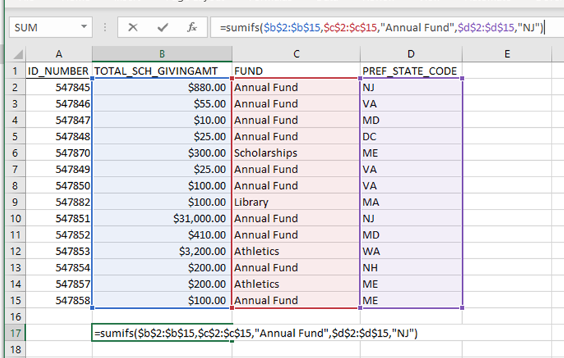
You can build your dashboard from a source file consisting of a list of gifts exported from your database. In our example below, the gift amount is in column B, the fund designation for each gift is in column C, and the donor’s state is in column D, listed in lines 2 through 1000.  Let’s break this formula into its constituent parts:

1. If we want the sum of gifts to the Annual Fund from New Jersey, our formula would look like =SUMIFS($b$2:$b$1000,$c$2:$c$1000,”Annual Fund”,$d$2:$d$1000,”NJ”).
   1. The first section (before the first comma) tells the =SUMIFS function that the data we want to sum is in the range from d2 to d1000.
   2. Because this range is static (i.e., it doesn’t change when we move or copy the cell to another location), we need to put dollar signs in front of the letter and number for each end of the range to tell it not to shift to the next row or column as we copy it down.
   3. The second and third sections ($c$2:$c$1000,”Annual Fund”) are the first set of criteria that make the function work:
      1. We are using the cell range 2-1000 for column C, which matches the sum range in column B; and
      2. Our filtering criterium is the text string “Annual Fund”.

• Then, the formula returns the sum of cells in column B where the field directly to the right in column C reads “Annual Fund.” The fourth and fifth sections filter further on column D and the text “NJ”.

These extremely powerful filters use the syntax criteria_range1, criteria1, criteria_range2, criteria2…; the =SUMIFS() and =AVERAGEIFS() also include a range which designates the numbers to be summed or averaged.  The criteria that you use for the “IFS portion of the command can include a simple text function (“Annual Fund”), a comparison (for example, “>=”&1000 for “greater than or equal to 1,000), or a reference to a cell (=b2).  Think of using it for:

• Finding Athletics donors who support cheerleading for the national competition in Florida
• Identifying $1,000+ donors
• Getting an average of membership levels, where membership is tracked on a different column in your worksheet from gift amounts.

​
Key Tip: For each function to work, the criteria range(s) and the sum or average range must start on the same line and end on the same line.

Think about using these functions on your detail worksheets in order to summarize data for a dashboard.
To find out more about the powerful uses of the tool that your office already has, find my other courses on the Staupell Website, here: https://www.staupell.com/business-intelligence-visualization-reporting.html
Feel free to write me at [email protected] with your ideas and questions.